excel chart with filter. Here is the basic data setup: The following example shows how to use this function in practice.
excel chart with filter Here are 4 methods for filtering your chart so you don’t have to edit or remove your data to get the perfect chart: Create a chart by selecting the whole dataset and choosing recommended charts. Select a cell from the data that is included in the chart and then go to the data tab and click the filter.


 & Dynamic Title on")


")


The Following Example Shows How To Use This Function In Practice.
Here is the basic data setup: Select a cell from the data that is included in the chart and then go to the data tab and click the filter. In this tutorial, you’ll learn how to apply filters to a chart in excel to display only the data you want.
Suppose We Have The Following Dataset In Excel That Shows The Sales Of Three Different Products During Various Years:
First, setup your data and create a chart that you want to use. Here are 4 methods for filtering your chart so you don’t have to edit or remove your data to get the perfect chart: In excel, the dynamic chart is a special type of chart that updates automatically when one or multiple rows are added or removed from the range or table.
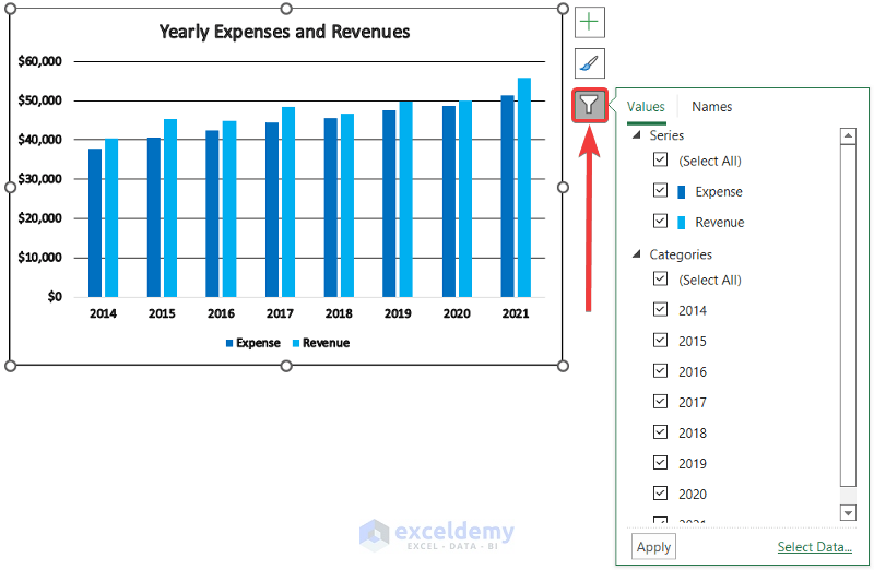
Often You May Want To Filter A Chart In Excel To Only Display A Subset Of The Original Data.
Fortunately this is easy to do using the chart filters function in excel. Create a chart by selecting the whole dataset and choosing recommended charts.